Table of Contents
- Introduction
- Transformer Network Architecture
- Perceptual Loss
- Training Specs
- Challenges Arising When Performing on Video
- Things to Experiment with Next Time
- Gallery
- References
1. Introduction
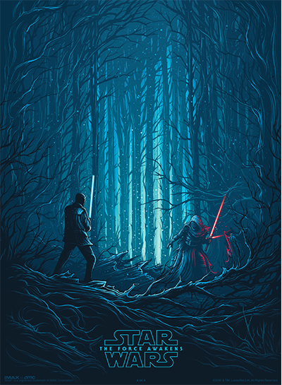
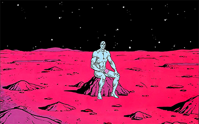
Neural style transfer is a deep learning technique that combines content and style of arbitrary images to create new artistic images (see Figure 1 or the Gallery). The technique was first introduced by Gatys et al. [1] and further refined by Johnson et al. [2] who introduced Perceptual Loss and framed the task as an image transformation problem rather than an optimization problem.
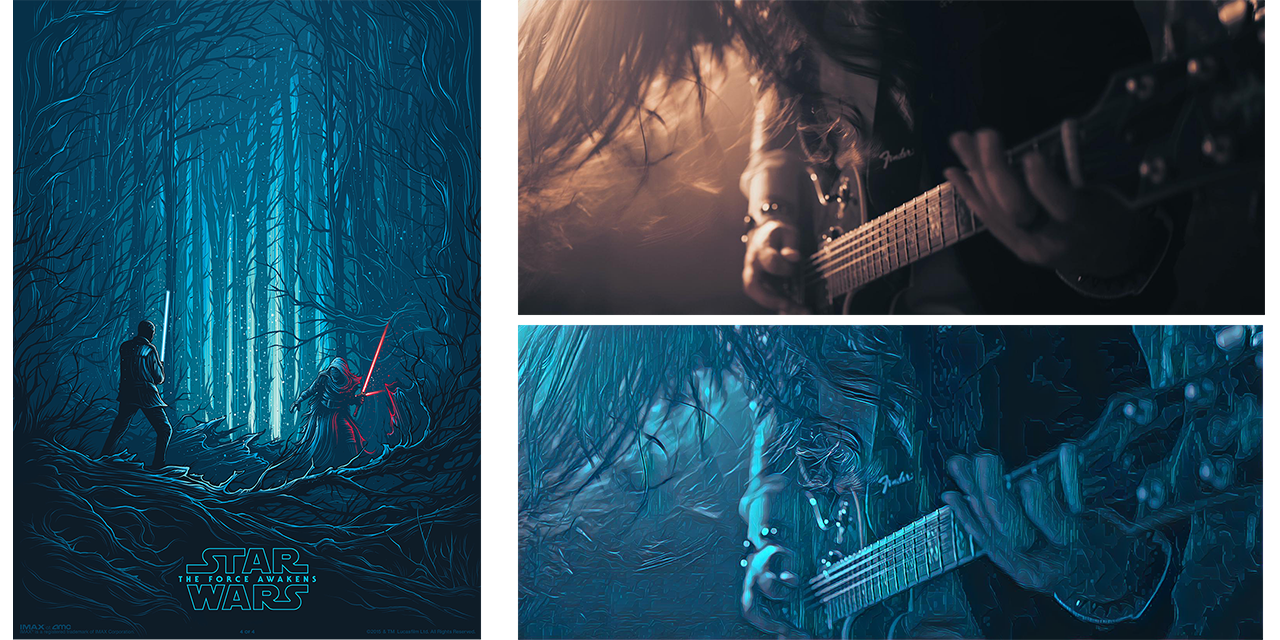
The general idea boils down to 2 components: the image transformation network and the loss network. The image transformation network inputs an image (the content image) and outputs a new (transformed) image. The loss network then quantifies how well the transformed image preserves the high-level features and spatial structure of the content image as well as how well it transfers the low-level properties (color, texture, shape etc.) of the style image. These notes use notation from [2] throughout.
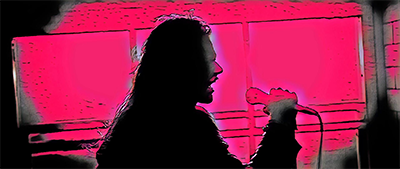
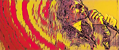
These are my condensed notes summarizing my brief dive into the topic of style transfer followed by an effort to create visual effects for the official music video for a song called Fly by the band Exit Empire:
2. Transformer Network Architecture
The original architecture of the transformer network proposed by [2][3] is described in Figure 2:
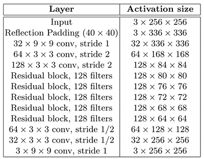
The transformer net we used differed slightly in a few implementation details. Rather than using Reflection padding (40 x 40) once in the beginning, smaller reflection padding prior to every convolutional layer was used to prevent the size reduction of the feature map. According to [8], using instance normalization instead of batch normalization improves the generated images. Every batch normalization was replaced with instance normalization in the architecture.
2.1 Instance Normalization
The simple difference between batch normalization and instance normalization is that batch normalization computes a single mean and standard deviation for the whole batch whilst instance normalization computes the mean and standard deviation for each element. In other words, BatchNorm normalizes the entire batch and InstanceNorm normalizes each image separately.
Or formally, in accordance with [8]:
Batch normalization:
$$\mu_i = \frac{1}{HWT}\sum_{t=1}^T\sum_{l=1}^W\sum_{m=1}^H x_{tilm}, \mu_i \in \mathbb{R}$$ $$\sigma_i^2 = \frac{1}{HWT}\sum_{t=1}^T\sum_{l=1}^W\sum_{m=1}^H (x_{tilm} - \mu_i)^2, \sigma_i \in \mathbb{R}$$
Instance normalization:
$$\mu_{ti} = \frac{1}{HW}\sum_{l=1}^W\sum_{m=1}^H x_{tilm}, \mathbf{\mu_i} \in \mathbb{R}^T$$ $$\sigma_{ti}^2 = \frac{1}{HW}\sum_{l=1}^W\sum_{m=1}^H (x_{tilm} - \mu_{ti})^2, \mathbf{\sigma_i} \in \mathbb{R}^T$$
Instance normalization is already implemented with most deep learning frameworks (PyTorch docs).
3. Perceptual Loss
Although not perfectly, style and content are separable in a convolutional neural network (CNN). Perceptual loss function measures high-level perceptual and semantic differences between images [2] using activations of intermediate layers in a loss network \(\Phi\). Most experiments use the pretrained VGG16 as the loss network.
Content loss is the Euclidean distance between the intermediate feature representations of the content image and the generated image. The higher the feature representation the more emphasis is given on high-level features and spatial structure in the resulting generated image rather than actual color, texture or shape. This encourages the generated image to be perceptually similar, but not necessarily match, the content image.
$$L_{content}(c, g) = \frac{1}{C_jH_jW_j}\left\lVert{\Phi_j(c) - \Phi_j(g)}\right\rVert_2^2$$
where \(c\) is the content image, \(g\) is the generated image, \(\Phi_j(x)\) is the \(j\)-th layer feature map of the loss network \(\Phi\) when processing image \(x\) and \(C_j, H_j, W_j\) are the number of channels, width and height of the feature map respectively. In our experiment, \(j=9\).
Speaking in code:
Style loss is the squared Frobenius norm of the differences between the Gram matrices of the style image and the generated image calculated at different layers (depths) of the loss network. The Gram matrix calculates the correlation between the feature maps, where width and height are flattened to a single dimension. This encourages the model to preserve stylistic features such as color, texture or shape.
Gram matrix is defined as the matrix of all possible inner products of vectors \(v_1, ..., v_m\); \(v_i \in \mathbb{R}^n\), i.e. a matrix \(\mathbf{G}\) of size \(m \times m\) where \(G_{ij}=\mathbf{v_i}^\top \cdot \mathbf{v_j}\). Let's denote:
$$G_j(x) = \frac{\overline{\Phi}_j(x) \overline{\Phi}_j(x)^\top}{C_jH_jW_j}$$
where \(G_j(x)\) is the Gram matrix \(\mathbf{G}_j\) for \(j\)-th layer feature map of loss network \(\Phi\) when processing image \(x\). Again, \(C_j, H_j, W_j\) are the number of channels, width and height of the feature map respectively. In the equation above, \(\overline{\Phi}_j(x)\) denotes the reshaped feature map of shape \(C_j \times H_jW_j\) (i.e. the width and height concatenated into a single dimension). The resulting Gram matrix \(\mathbf{G}_j\) thus has a shape of \(C_j \times C_j\).
Speaking in code (PyTorch):
Style loss can then be defined as:
$$L_{style}(s, g) = \sum_{j \in J} \left\lVert{G_j(s) - G_j(g)}\right\rVert_F^2$$
where \(s\) is the style image, \(g\) is the generated image. Notice the sum across a set of layers \(J\). In the case of VGG16 as the loss network \(\Phi\), we set \(J = \{4, 9, 16, 22\}\). The notation above uses Frobenius norm which is equivalent to the Euclidean norm generalized to matrices instead of vectors.
Speaking in code:
The total loss is then the sum of the content loss and the style loss each weighted by a hyper parameter to balance the trade-off between the content or the style.
$$L_{total}(c, s, x) = \alpha L_{content}(c, g) + \beta L_{style}(s, g)$$
The provided code examples are simplified for a demonstration purposes, for actual implementation it is recommended to calculate the loss in batches.
4. Training Specs
We used COCO training set 2014 as training data [6]. Things we tried:
- The choice of optimizer had little effect on the quality of the generated images. Choose Adam.
- 2 epochs worked perfectly fine. 1 epoch was not enough, 3 were too much.
- Similarly to [2], we trained on images of size 256 x 256. Training on larger images (299 x 299, 384 x 384) had little to no effect on the resulting quality of the images whilst trained longer.
- Ironically, extending the COCO training dataset with the frames of the video deteriorated the quality of the final outcome.
- Setting style loss weight equal to double of the content style loss weight seemed to be the right balance. Although varied a little based on the style image.
- Scaling or normalizing input images also slightly deteriorated the generated images.
- Storing images resized and as 8-bit integers enabled us to fit all the training data into memory as one big tensor rather then loading them from file with each batch. Using a prefetcher to perform conversion to torch.Tensor, loading to GPU and casting to 32-bit float (once on the GPU) in a separate CUDA stream (i.e. performed simultaneously with training for the next batch) sped things up even further.
5. Challenges Arising When Performing on Video
When performing style transfer on video, a few challenges arise. First of all, consecutive frames can differ too much in a way that creates an undesired effect. Despite some efforts to make style transfer consistent on video sequences [7] by introducing additional penalty to the loss function, we found using appropriate style images to be a sufficient "hack".
In scenarios where the resulting video quality is of high importance, using the right library to write frames into a video file in lossless quality is crucial. (You can always decrease the quality during final cut, however, you cannot go the other way.) OpenCV did not quite cut it, however, using any FFMPEG wrapper should enable to render the video without any compression and hence work fine, provided that you set the right settings. We used MoviePy and overwrote a couple of the default settings in the source code for lossless quality, namely:
- Change the Constant Rate Factor ("crf") to 0 (see reference).
- Change the Pixel Format ("pix_fmt"), i.e. YUV to YUV422 (8bytes per 4 pixels) from the default YUV420p (6bytes per 4 pixels). Ideally, we would have used YUV444 (12bytes per 4 pixels), however, we ran into problems opening videos exported with YUV444 in a video editing software.
Note: in the case of MoviePy, we're talking about changing these lines.
You can download the whole music video rendered in lossless quality for free here.
6. Things to Experiment with Next Time
- Network architecture inspired by U-Net.
- Dense blocks instead of residual blocks.
- Train on ImageNet subset.
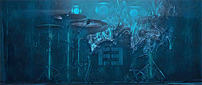
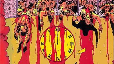
7. Gallery


References
| [1] | Gatys, Leon A., Alexander S. Ecker, and Matthias Bethge. "A Neural Algorithm of Artistic Style." arXiv preprint arXiv:1508.06576 (2015). URL |
|---|---|
| [2] | Johnson, Justin, Alexandre Alahi, and Li Fei-Fei. "Perceptual Losses for Real-Time Style Transfer and Super-Resolution" European Conference on Computer Vision. Springer, Cham, 2016. URL |
| [3] | Johnson, Justin, Alexandre Alahi, and Li Fei-Fei. "Perceptual Losses for Real-Time Style Transfer and Super-Resolution": Supplementary Material. Technical report. URL |
| [4] | Joshi, Bhautik, Kristen Stewart, and David Shapiro. "Bringing Impressionism to Life with Neural Style Transferin Come Swim." Proceedings of the ACM SIGGRAPH Digital Production Symposium. ACM, 2017. URL |
| [5] | Li, Yijun, et al. "A Closed-form Solution to Photorealistic ImageStylization." arXiv preprint arXiv:1802.06474 (2018). URL |
| [6] | Lin, Tsung-Yi, et al. "Microsoft COCO: Common Objects in Context." European conference on computer vision. Springer, Cham, 2014. URL |
| [7] | Ruder, Manuel, Alexey Dosovitskiy, and Thomas Brox. "Artistic Style Transfer for Videos." German Conference on Pattern Recognition. Springer, Cham, 2016. URL |
| [8] | Ulyanov, D., A. Vedaldi, and V. S. Lempitsky. "Instance Normalization: The Missing Ingredient for FastStylization" arXiv preprint arXiv:1607.08022 (2016). URL |